The differential equation (2.7) from the last topic is utilized to describe the process of diffusion under the prescribed conditions in Figure 2.5 (last post, post 2.4). The following boundary conditions or hypothesis should be assumed in this case:
1 – For t=0 , C = C0 for \( 0\leq x\leq\infty \)
2 – For t > 0, C = Cs for x = 0 and C = C0 for \(x=\infty\)
The differential equation solution (2.7), applied to these boundary conditions is the following: \[ \frac{C_{x}-C_{0}}{C_{S}-C_{0}}= 1 – erf (\frac{x}{2\sqrt{Dt}}) \tag{2.8} \]
The function \( erf(z)=(\frac{X}{2\sqrt{Dt}}) \) is a normalized probability integer or Gauss1 error function. The Gauss error function is defined as: \[ erf (z) = \frac{2}{\sqrt{\pi}} \int_{0} ^{z} e ^{- y^{2}}dy \tag{2.9} \]
where \( \frac{X}{2\sqrt{Dt}} \) is the variable z.
The values of the Gaussian Error Function z=erf(y), like other common mathematical functions are tabulated (see table below) .
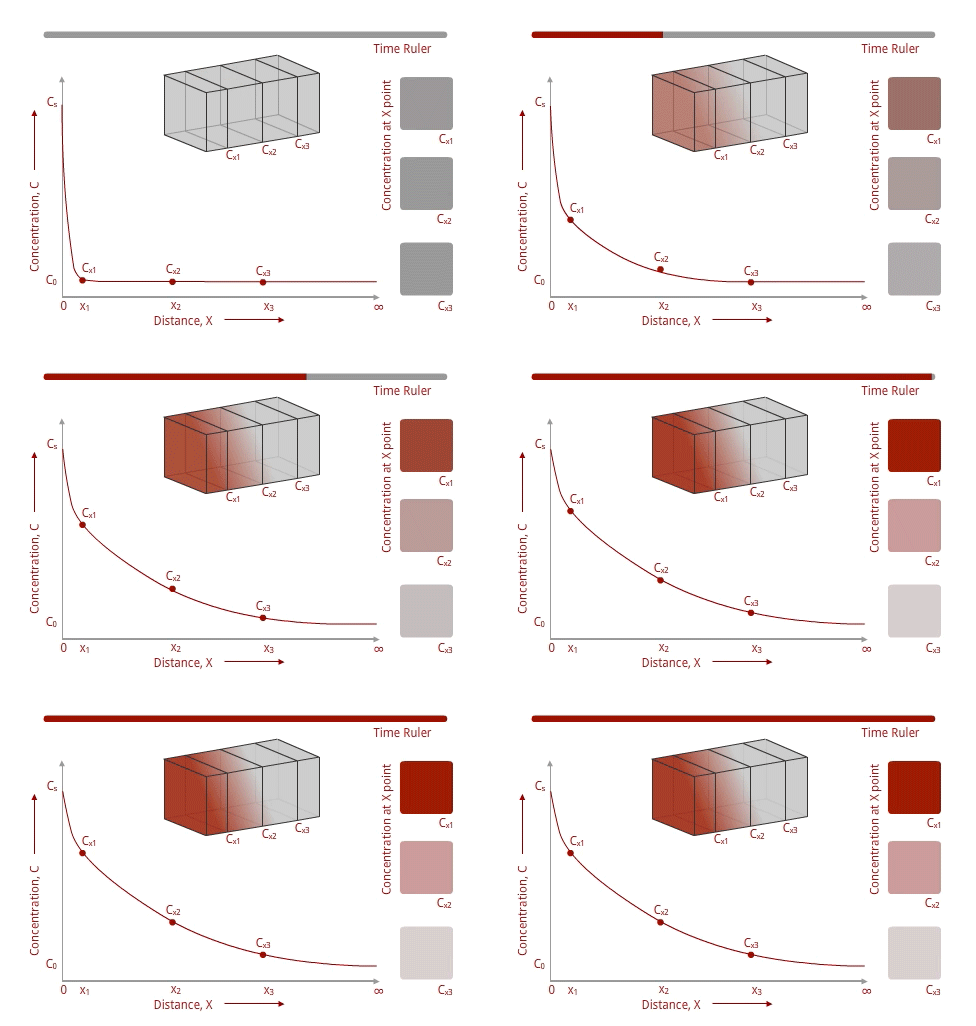

The importance of the curve shown in Figure 2.2.6 (see below) is in the interrelationship between distance, time, the diffusion coefficient, and the concentration during diffusion. If C0, CS and D were known of a material, CX should be a function of the adimensional parameter (x/√Dt) . If we wish to double the depth of penetration, the diffusion time should be four times greater. In general, for a depth n times greater than the original, the diffusion time should be multiplied by n2. The variations in the diffusion coefficient are equivalents to the variations in the diffusion time, e.g., if D is doubled, only half the time would be required to reach the same depth of penetration. To produce a determined concentration in a certain region of material or to spread throughout the material a certain fraction of the necessary quantity for total saturation, simply maintain at the same value L/√Dt, in which L is a dimension that characterizes the size of the object.
 Figure 2.2.6 – Use of the Gauss error function in diffusion.
1Johann Carl Friedrich Gauss (1777 – 1855), german mathematician and scientist with important contributions in mathematics, astronomy, optics, electrostatics, etc.