When the concentration of the species in diffusion varies over time, this diffusion species will accumulate within the volume. Under transitory, transient or non-steady state conditions, the gradient \( \frac{dC}{dx} \) and, therefore, the flux J of Eq. (2.2), vary over time. This is illustrated in Figure 2.2.3, that shows the concentration profiles taken in three different instances in time t1, t2, t3.

The concentration variation can be determined over time, during the diffusion process, for any given point in the interior of a solid, by determining the difference between the flux that enters and leaves of an element by volume. If two parallel planes separated by a distance dx were considered, like in the illustration in Figure 2.2.4, the flux that enters the first plane is
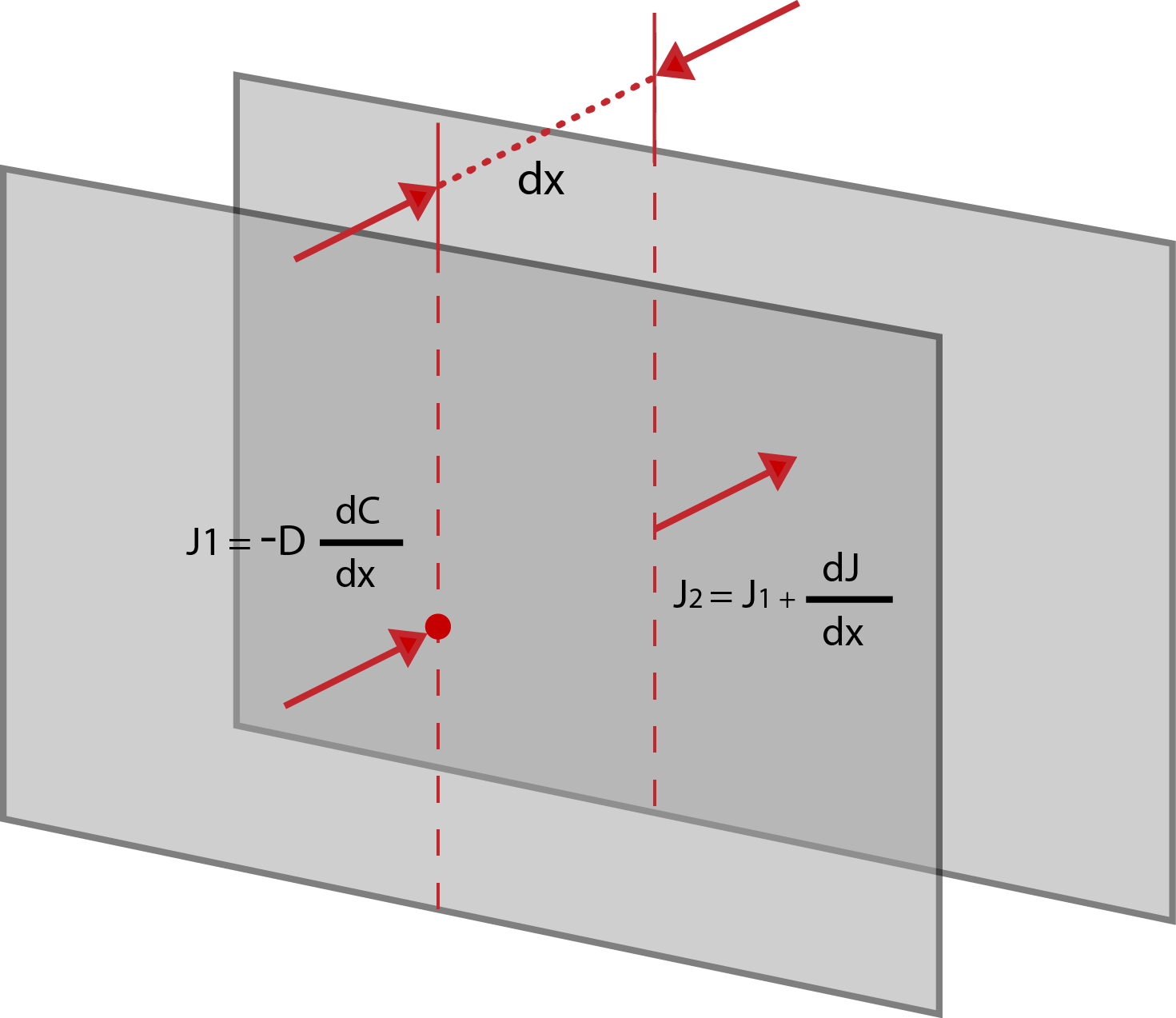
\[ J _ {1} =-D \frac{\partial C}{\partial x} \tag{2.3} \]
and the flux through the second plane is
\[ J _ {2} =J + \frac{\partial J}{\partial x} dx \tag{2.4} \]
Subtracting J1 – J2, we get:
\[ \frac{\partial J}{\partial x} = – \frac{\partial }{\partial x} [D \frac{\partial C}{\partial x}] \tag{2.5} \]
The variation of the flux with the distance is equal to
\[ -\frac{\partial C}{\partial t}\]
From there we get Fick’s Second Law:
\[ \frac{\partial C}{\partial t} = \frac{\partial }{\partial x} [D \frac{\partial C}{\partial x}] \tag{2.6} \]


